This section describes the procedure for constructing a reference (baseline) model, which provides the initial quality metrics and ensures correct data preparation, model configuration, and parameter settings for further training steps.

The reference model is created by excluding background pixels from hyperspectral images, allowing for automatic segmentation of disease-affected regions in plant samples.

It serves as a foundational template applied uniformly across all images to support training and classification tasks.

The process begins by adding a new segmentation and assigning it a name (Figures 39, 40).

The model creation wizard then guides through the following function-based steps:

1) Selecting the measurements for segmentation (Figure 41);

2) Choosing spectral bands within defined wavelength ranges - typically covering the entire spectrum with SNV preprocessing applied by default - including:

- raw spectral data for segmentation (Figure 42);

- model loadings corresponding to principal components (Figure 43);

- signal-to-noise ratio across the wavelength range (Figure 44);

3) Pixel selection involves:

- obtaining a mosaic of images (Figure 45);

- identifying Regions of Interest (ROI) that contain pixels representing diseased areas, usually indicated by bright colours (mainly red and yellow) clustered in scatter plots. Pixel inclusion or exclusion is controlled via the toolbar on the right, which also offers tools to remove boundary pixels if needed (Figures 46, 47, 48)

4) Defining a critical distance threshold to determine pixel association with the reference model. The histogram of these distances encompasses all pixels, with an adjustable red threshold line set to isolate only pixels associated to diseased regions while excluding background (Figure 49, 50);

5) The reference model is finalised by setting a minimum region size (typically around 300 pixels) to filter out noise. This value can be adjusted depending on the size of the regions of interest and prior pixel selections. After completion, the reference model is automatically applied to the image dataset (Figure 51).

Using this baseline model enables clear visualisation of segmented, unique disease-affected regions on plant samples (Figure 52, 53).

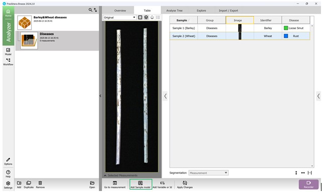
Figure 39 – Addition of a reference model

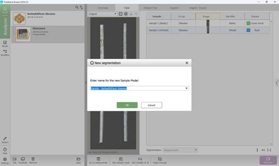
Figure 40 – Adding a new segmentation and assigning a name to the reference model

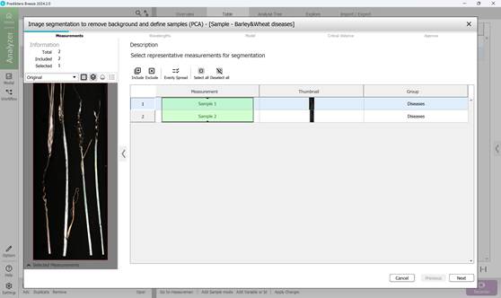
Figure 41 – Measurement selection for segmentation

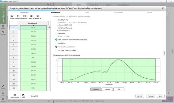
Figure 42 – Raw Spectrum of measurements for segmentation

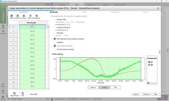
Figure 43 – Model loadings on principal components

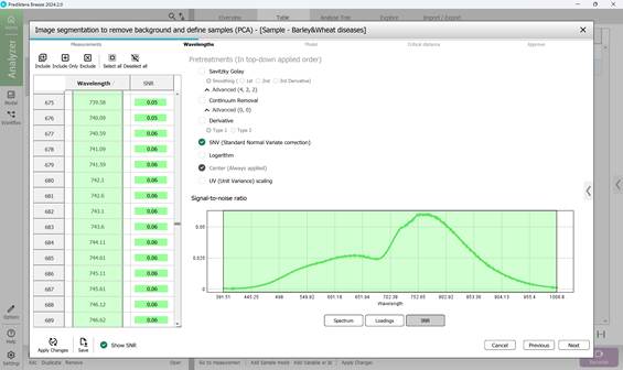
Figure 44 – Signal-to-noise ratio across the wavelength range

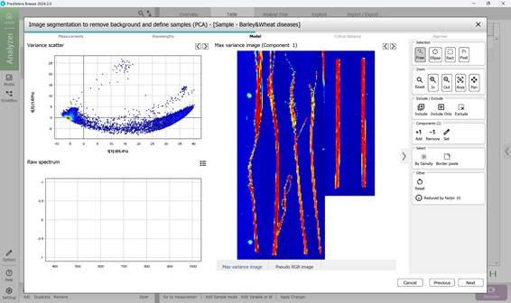
Figure 45 – Mosaic of images and PCA model based on mosaic pixels

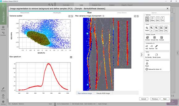
Figure 46 – Pixel and corresponding point selection in a Variance Scatter cluster

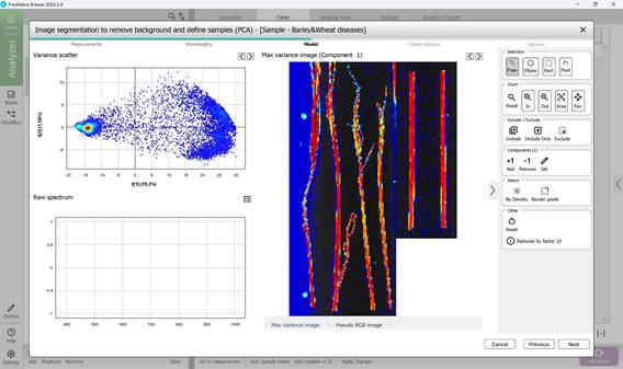
Figure 47 – Intermediate result of excluding pixels outside regions of interest (ROI)

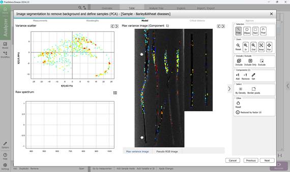
Figure 48 – Selecting subregions of ROIs

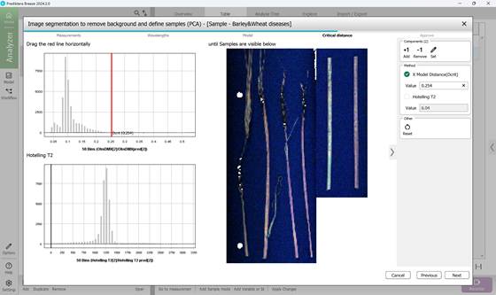
Figure 49 – Determining the threshold of critical distance

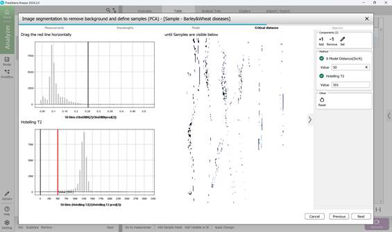
Figure 50 – Determination of critical distance threshold metrics corresponding to ROIs

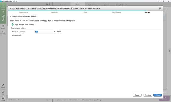
Figure 51 – Completion of reference model creation: verification of the minimum area size in pixels and its application to project images

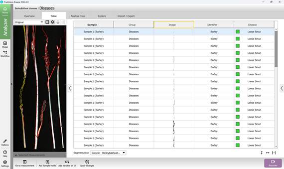
Figure 52 – Identification and visualisation of Loose smut-affected crop regions using the reference model

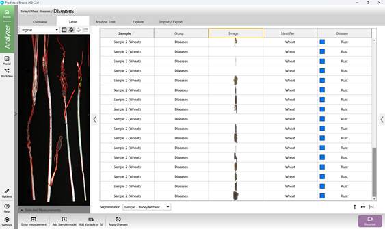
Figure 53 – Identification and visualisation of Brown rust-affected crop regions using the reference model