This section discusses the application of the trained classification model for diagnosing crop diseases based on hyperspectral data.

In order to fully integrate the classification model into the workflow algorithm, it needs to be inserted into the “Analyse Tree” by using the “Add node” button (Figure 72). This functionality enables the integration of different models, parameters, and metrics into the current algorithm. Selecting the “Add node” option opens a window that lists the available tools for addition. The classification model can be added by selecting the “Classification of Categories” option, which is located in the “Model” tools subgroup (Figure 73).

After selection, the tool is added to the Analysis Tree and presents options for identifying crop diseases, each represented by distinct colours. These colours correspond to the highlights used to mark affected regions on hyperspectral images. The right-hand panel provides information about the included model, such as model type, classification feature, classification technique, and additional details (Figure 74).

To run the algorithm across all samples, the modifications to the current analysis must be confirmed by clicking the “Apply Changes” button on the bottom panel (Figure 75). Once changes are applied, the trained classification model automatically assigns disease categories to infected crop samples, including “Loose Smut” (Figure 76) and “Brown Rust” (Figure 77).

Figure 72 – Analysis Tree modeling

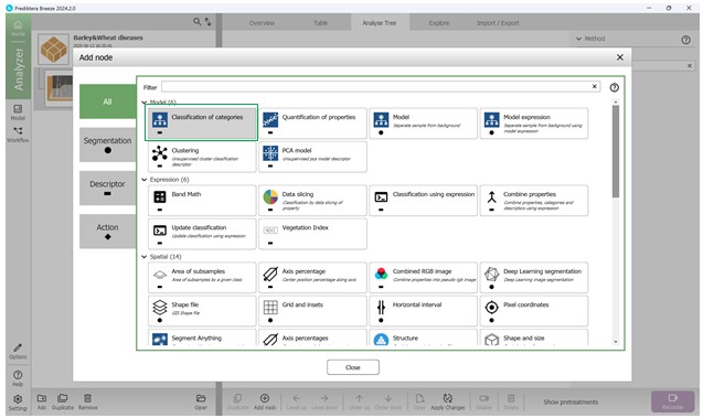
Figure 73 – Adding a node to the tree to build a visual hierarchy of analysis

Moreover, the software allows for the measurement of morphometric features of infected regions, including area, length, width, perimeter, and the roundness coefficient. Additional metrics may be added into the Analysis Tree by clicking the “Add node” button, available either within the classification model or on the lower panel (Figure 78).

Figure 74 – Adding a previously created classification model as a tree node

Figure 75 – Applying the changes made to the current analysis stages

Figure 76 – Classification of trained samples on “Loose smut” disease following analysis updates

Figure 77 – Classification of trained samples on “Brown rust” disease following analysis updates

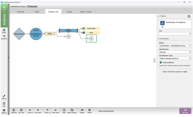
Figure 78 – Adding supplementary metrics to the Analysis Tree

Next, within the tool options window, choose the metric group labelled “Shape and Size” (Figure 79). After selection, this metric will be listed as “Area (mm)” in the Analysis Tree. It is possible to modify the measurement units and other configurations in the “Parameters” panel located on the right side (Figure 80). The “Output” setting enables selection of the exact metric, such as “Area” (Figure 81). To include an additional metric from the same category in the Analysis Tree, the “Add node” button may be used, or the “Duplicate” feature may be selected by right-clicking (Figure 82). These settings support different units, including pixels, which are useful for measuring damage extent.

For plant specimens, it is also possible to compute vegetation indices. This involves clicking on “Add node” and choosing an index (e.g., NDVI) from the “Vegetation Index” category to include it in the Analysis Tree (Figures 83, 84). The NDVI index indicates the photosynthetic activity level and aids in detecting stress conditions.

Once particular metrics are added to the algorithm, corresponding empty columns are created to display the calculated values for the relevant regions under analysis. To compute and show these values for each sample and metric, the modifications to the algorithm need to be confirmed by pressing the “Apply Changes” button (Figure 85).

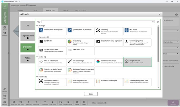
Figure 79 – Selecting the “Shape and Size” metrics category to add to the Analysis Tree

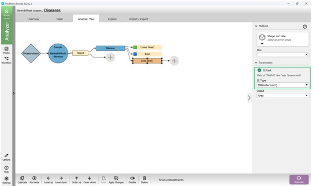
Figure 80 – Adding the “Area” metric to the Analysis Tree and selecting the unit of measurement

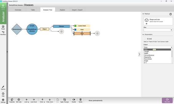
Figure 81 – Selecting the output parameter for the added metric

Figure 82 – Adding a new metric to the Analysis Tree by means of the “Duplicate” option

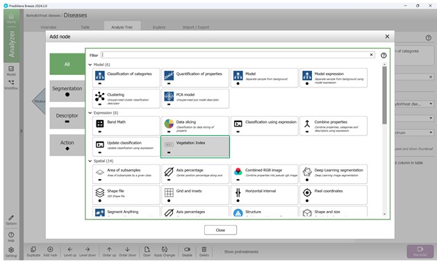
Figure 83 – Selecting the “Vegetation Index” category of metrics to add to the Analysis Tree

Figure 84 – Adding the NDVI index to the Analysis Tree

The results of applying the trained model for classifying infected regions of crops for signs of “Loose smut” disease (Figure 86) and “Brown Rust” disease (Figure 87) are displayed in previously created columns.

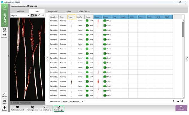
Figure 85 – Sample columns based on metrics added to the Analysis Tree

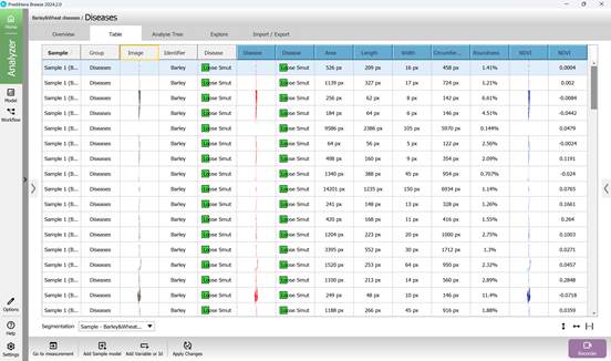
Figure 86 – Classification results of infected crop regions for “Loose smut” disease using the trained model

Figure 87 – Classification results of infected crop regions for “Brown rust” disease using the trained model

Hyperspectral imaging enables highly accurate detection of infected regions for diagnosing plant diseases based on their spectral characteristics using machine learning methods. This approach allows identification of stress indicators in crops at various developmental stages, including early ones, significantly enhancing the effectiveness of crop condition monitoring.